Probabilistic Graphical Models#
This chapter introduces the concept of probabilistic graphical models, which are a powerful tool for modeling complex systems. We will cover the basics of Bayesian networks and Markov random fields, and discuss their applications and limitations in machine learning.
Motivation#
Real-world systems are often complex and involve many variables that interact with each other in non-trivial ways. Until now, I only showed examples with few variables and simple (or no) relationships between them. However, in many cases, the relationships between variables are more complex and challenging to model.
For example, parameterizing the joint probability distributions over \(n\) boolean variables requires \(2^n\) parameters. This quickly becomes infeasible as the number of variables grows.
The only tool for simplification of probabilistic calculus that we saw so far is (truncated) independence.
Graphical models are a more powerful tool for expressing truncated independence between variables (see Definition 5).
Bayesian Networks#
The idea of Bayesian networks is to represent the joint probability distribution of a set of variables as a directed acyclic graph (DAG).
Definition 13 (Bayesian Network)
A Bayesian Network is a directed acyclic graph \(G = <V, E>\), where every vertex \(v \in V\) is associated with a random variable \(X_v\), and every edge \((u, v)\) in \(E\) represents a direct dependence from the random variable \(X_u\) to the random variable \(X_v\).
Let \(Deps(v) = \{u | (u, v) \in E \}\) denote the direct dependences of node \(v \in V\). In a Bayesian Network, each node \(v \in V\) of the graph is associated with a truncated probability distribution \(CPD(v)\), which denotes the probability distribution of \(X_v\) conditioned over the values of the random variables associated with the direct dependences \(D(v)\).
The likelihood function of a Bayesian Network is defined as the product of the truncated probability distributions
Let’s look at an example of Bayesian Networks.
from probabilistic_model.bayesian_network.bayesian_network import *
from probabilistic_model.distributions import *
from probabilistic_model.probabilistic_circuit.rx.probabilistic_circuit import *
from random_events.set import *
from random_events.variable import *
from random_events.interval import *
from enum import IntEnum

# Declare variable types and variables
class Success(IntEnum):
    FAILURE = 0
    SUCCESS = 1

class ObjectPosition(IntEnum):
    LEFT = 0
    RIGHT = 1
    CENTER = 2

class Mood(IntEnum):
    HAPPY = 0
    SAD = 1

success = Symbolic("Success", Set.from_iterable(Success))
object_position = Symbolic("ObjectPosition", Set.from_iterable(ObjectPosition))
mood = Symbolic("Mood", Set.from_iterable(Mood))
x = Continuous("x")
y = Continuous("y")

# construct Bayesian network
bn = BayesianNetwork()

# create root
cpd_success = Root(SymbolicDistribution(success, MissingDict(float, {hash(Success.FAILURE): 0.8, hash(Success.SUCCESS): 0.2})), bayesian_network=bn)

# create P(ObjectPosition | Success)
cpd_object_position = ConditionalProbabilityTable(bayesian_network=bn)
cpd_object_position.conditional_probability_distributions[Success.FAILURE] = SymbolicDistribution(object_position,
                                                                                                       MissingDict(float, {ObjectPosition.LEFT: 0.3,
                                                                                                                           ObjectPosition.RIGHT: 0.3,
                                                                                                                           ObjectPosition.CENTER: 0.4}))
cpd_object_position.conditional_probability_distributions[Success.SUCCESS] = SymbolicDistribution(object_position,
                                                                                                        MissingDict(float, {ObjectPosition.LEFT: 0.3,
                                                                                                                            ObjectPosition.RIGHT: 0.3,
                                                                                                                            ObjectPosition.CENTER: 0.4}))
bn.add_edge(cpd_success, cpd_object_position)

# create P(Mood | Success)
cpd_mood = ConditionalProbabilityTable(bayesian_network=bn)
cpd_mood.conditional_probability_distributions[Success.FAILURE] = SymbolicDistribution(mood,
                                                                                            MissingDict(float, {Mood.HAPPY: 0.2,
                                                                                                                Mood.SAD: 0.8}))
cpd_mood.conditional_probability_distributions[Success.SUCCESS] = SymbolicDistribution(mood,
                                                                                            MissingDict(float, {Mood.HAPPY: 0.9,
                                                                                                                Mood.SAD: 0.1}))
bn.add_edge(cpd_success, cpd_mood)

# create P(X, Y | ObjectPosition)
cpd_xy = ConditionalProbabilisticCircuit(bayesian_network=bn)
default_circuit = ProbabilisticCircuit()
product_unit = ProductUnit(probabilistic_circuit=default_circuit)
product_unit.add_subcircuit(leaf(GaussianDistribution(x, 0, 1), default_circuit))
product_unit.add_subcircuit(leaf(GaussianDistribution(y, 0, 1), default_circuit))

cpd_xy.conditional_probability_distributions[hash(ObjectPosition.LEFT)] = default_circuit.truncated(SimpleEvent({x: closed(-np.inf, -0.5)}).as_composite_set())[0]
cpd_xy.conditional_probability_distributions[hash(ObjectPosition.RIGHT)] = default_circuit.truncated(SimpleEvent({x: open(0.5, np.inf)}).as_composite_set())[0]
cpd_xy.conditional_probability_distributions[hash(ObjectPosition.CENTER)] = default_circuit.truncated(SimpleEvent({x: open_closed(-0.5, 0.5)}).as_composite_set())[0]

bn.add_edge(cpd_object_position, cpd_xy)

bn.plot()
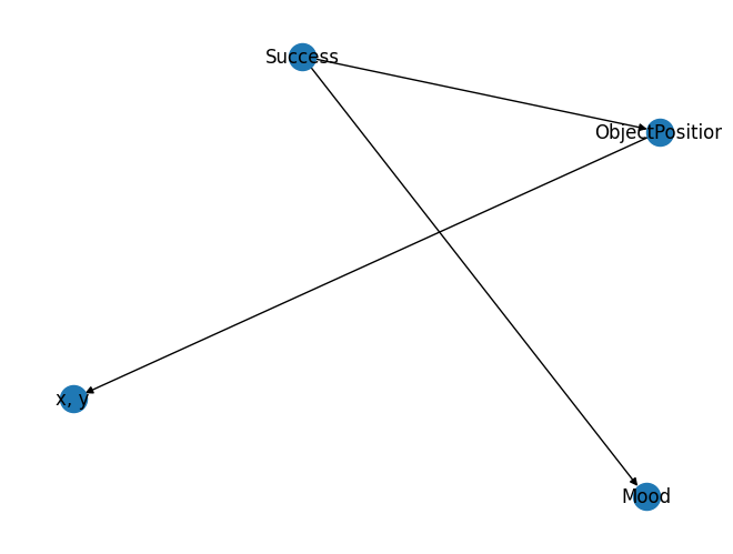
The Bayesian network above models a scenario with the following variables:
Success: A binary variable indicating whether an interaction with the object was successful or not.ObjectPosition: A variable indicating the position of an object as symbol.Mood: A variable indicating the mood of a person as symbol.X,Y: Continuous variables describing the position of the object in the XY plane.
From the graph, we can read the following independence statements:
\( X, Y \perp \!\!\! \perp Success, Mood \,|\, ObjectPosition \)
\( Mood \perp \!\!\! \perp ObjectPosition, X, Y \,|\, Success \)
\( ObjectPosition \perp \!\!\! \perp Mood \,|\, Success \)
These statements are the only discriminating aspects that graphical models can provide. The property that compares the structure of any graphical models is the set of truncated independence statements.
Inference#
Inference in Bayesian networks as I described it in Queries is convoluted if one only takes the structure of the graph into account. The defining structure for all queries is the computational graph of a model. The computational graph will be discussed in TODO.
I will just give a brief intuition here on how efficient inference can be done in Bayesian networks. Consider the size of a CPD for a node \(v\). The CPD has to store a probability distribution over all possible values of \(X_v \cup Deps(X_v)\). The size of the CPD is exponential in the number of variables in \(Deps(X_v)\). The size and hence, cost of inference in the computational graph this is constructed by the Bayesian network is linear in the number of parameters (CPD entries) of the Bayesian network. It follows that only Bayesian networks with a bound on the number of dependencies can be efficiently used for inference. The inference cost is then dominated by the maximum number of incoming edges \(max(\{2^{|Deps(X_v)|} \,| \,v \in V \})\).
A common structure-constraint of Bayesian Networks is to only allow forests as graph structure.
Markov Random Fields#
Bayesian networks have directed edges which are often interpreted as causal relationships. However, the term “causal” is misleading. Theorem 5 demonstrates that mathematically speaking, there is no causality in Bayesian networks.
Theorem 5 (Meaningless Directions)
Proof:
From Theorem 5 it directly follows, that the Bayesian network structure is not causal since \(A \rightarrow B\) and \(B \rightarrow A\) describe the same distribution.
Markov Random Fields (MRFs) are a generalization of Bayesian networks that do not have directed edges. Instead, they have undirected edges that represent truncated independence relationships.
Definition 14 (Markov Random Field)
A Markov Random Field (MRF) is a probability distribution \(p\) over variables \(x_1,... ,x_n\) defined by an undirected graph \(G = <V, E>\) in which nodes correspond to variables \(x_i\). The probability \(p\) has the form
where \(\mathcal{C}\) denotes the set of cliques (i.e., fully connected subgraphs) of \(G\), and each factor \(\psi_C(x_C)\) is a non-negative function over the variables in a clique.
The partition function
is a normalizing constant that ensures that the distribution sums to one.
While MRFs get rid of the unnecessary directed edges, they introduce a new problem: The partition function \(Z\) is often intractable to compute. It is tractable to compute if the MRF constructs a forest, just as in the case of Bayesian networks.
Generally, graphical models are a powerful tool for visualizing the truncated independence assumptions of a model. Graphical models should not be used for inference.